Everything about loss functions that actually comes up in interviews, and nothing that doesn’t.
Read the table, then go deep only where you’re shaky. Every section ends with the trap interviewers use to find out whether you’ve actually shipped a model.
1. The 60-Second Table
If you remember nothing else, remember this.
| Task | Loss | Core idea | PyTorch |
|---|---|---|---|
| Binary classification | BCE | Likelihood of correct class | BCEWithLogitsLoss |
| Multiclass (one label) | Softmax + CE | Likelihood of correct class | CrossEntropyLoss |
| Multilabel | Per-label sigmoid + BCE | Labels are independent | BCEWithLogitsLoss |
| SVM / margin | Hinge | Margin, not probability | MultiMarginLoss |
| Regression | MSE (L2) | Penalize squared error | MSELoss |
| Robust regression | MAE (L1) / Huber | Reduce outlier pull | L1Loss / HuberLoss |
| Class imbalance | Focal, weighted BCE | Down-weight easy examples | pos_weight= |
| Ranking | Pairwise / listwise | Relative order | MarginRankingLoss |
| Similarity | Contrastive | Pull similar, push apart | CosineEmbeddingLoss |
| Metric learning | Triplet | Positive closer than negative | TripletMarginLoss |
| Dense retrieval | InfoNCE | Positive vs many negatives | in-batch softmax |
| Distribution matching | KL | Match distributions | KLDivLoss |
| LLM pretraining | Token CE | Predict next token | CrossEntropyLoss |
| SFT | Token CE (masked) | Predict response only | ignore_index=-100 |
| Distillation | KL + CE | Match teacher’s soft targets | KLDivLoss |
| Preference tuning | DPO | Preferred beats rejected | custom |
| RLHF | Reward - KL penalty | Maximize reward, stay near ref | custom |
The four relationships that cover most questions:
$$\text{Classification} \rightarrow \text{Cross-Entropy} \qquad \text{Regression} \rightarrow \text{MSE / MAE / Huber}$$$$\text{Ranking} \rightarrow \text{Pairwise / Listwise} \qquad \text{Embeddings} \rightarrow \text{Contrastive / Triplet / InfoNCE}$$2. The Foundation
A loss measures how far a prediction \(\hat y\) is from the target \(y\). Training minimizes it over the parameters \(\theta\):
$$\theta^* = \arg\min_\theta \frac{1}{N}\sum_{i=1}^{N} L(y_i,\hat y_i), \qquad \theta \leftarrow \theta - \eta\nabla_\theta L$$Loss vs cost vs objective. Loss is the error on one example, cost is the average over a batch or dataset, and the objective is what you actually optimize, which may add regularization:
$$J(\theta)=\frac{1}{N}\sum_i L_i + \lambda R(\theta)$$People use these interchangeably in conversation. Knowing the distinction is worth one clean sentence in an interview, not an argument.
By convention we minimize losses. The same quantity negated and maximized is called a utility or reward function, which is why RLHF talks about maximizing reward while everything else talks about minimizing loss. It is a sign convention, not a different idea.
The requirement that matters: the loss must be differentiable with respect to the parameters (almost everywhere). That single constraint explains most of what follows, including why we never put argmax in a training loss.
3. Classification
3.1 Binary Cross-Entropy
The model outputs a logit \(z\), squashed to a probability \(p=\sigma(z)=1/(1+e^{-z})\). For \(y\in\{0,1\}\):
$$L=-[y\log p+(1-y)\log(1-p)]$$Intuition. BCE punishes being confident and wrong. With \(y=1\): \(p=0.9\) is a small loss, \(p=0.1\) is a large one, and \(p=0.001\) is enormous. The log is what makes confident mistakes so expensive, and it is exactly what connects BCE to maximum likelihood, since minimizing \(-\log P(y \mid x)\) is maximizing \(P(y \mid x)\).
Trap: use
BCEWithLogitsLoss, notSigmoidfollowed byBCELoss. The fused version applies the log-sum-exp trick and stays stable when logits are large; the manual version silently producesinfornan. If someone shows you training code with a sigmoid feedingBCELoss, that is the bug they’re asking about.
3.2 Multiclass Cross-Entropy
For \(K\) mutually exclusive classes, softmax turns logits into probabilities and CE scores the correct one:
$$p_k=\frac{e^{z_k}}{\sum_j e^{z_j}}, \qquad L=-\sum_{k=1}^{K}y_k\log p_k = -\log p_c$$The last equality is the useful one: with a one-hot target, cross-entropy is just the negative log probability of the correct class \(c\). Every other term is multiplied by zero.
Say this precisely: softmax is an activation, cross-entropy is the loss. “Softmax loss” is informal shorthand for the pair.
Terminology: cross-entropy, negative log-likelihood (NLL), and log loss all name the same quantity. Keras says categorical cross-entropy for the multiclass case and binary cross-entropy for two classes; PyTorch says
CrossEntropyLossandBCEWithLogitsLoss. Interviewers switch between these names without warning, so treat them as synonyms.
Trap:
nn.CrossEntropyLossalready applieslog_softmaxinternally. Feeding it softmax outputs applies softmax twice, which flattens your gradients and quietly hurts accuracy. It also expects class indices, not one-hot vectors. This is the single most common PyTorch bug in interview code-review questions.
Why not argmax before the loss? Argmax has zero gradient almost everywhere and is undefined at ties, so nothing would propagate. Train on continuous probabilities, use argmax only at inference to produce a discrete label.
3.3 Binary vs Multiclass vs Multilabel
| Type | Target | Output layer | Loss |
|---|---|---|---|
| Binary | \(y\in\{0,1\}\) | 1 logit, sigmoid | BCE |
| Multiclass | exactly one of \(K\) | \(K\) logits, softmax | CE |
| Multilabel | any subset of \(K\) | \(K\) logits, sigmoid each | BCE per label |
An image tagged {dog, outdoor, grass} is multilabel. Softmax is wrong here because it forces the probabilities to sum to 1, making the labels compete when they should be independent.
Trap: “multiclass vs multilabel” is a favorite because the fix is one line (softmax to sigmoid) but the symptom is subtle: the model can never confidently predict two tags at once.
3.4 Label Smoothing
Instead of a hard target of 1 for the correct class, use \(1-\epsilon\) and spread \(\epsilon\) across the rest:
$$y_k^{LS} = (1-\epsilon)y_k + \frac{\epsilon}{K}$$Hard targets push the correct logit toward infinity, which produces overconfident, poorly calibrated models. Smoothing caps that pressure and usually improves generalization and calibration. It costs one argument: CrossEntropyLoss(label_smoothing=0.1).
Trap: it hurts when you need the raw probabilities downstream, as in distillation or retrieval calibration, because it deliberately distorts them.
3.5 Hinge Loss
The SVM objective, with \(y\in\{-1,+1\}\):
$$L=\max(0,1-y f(x))$$Once \(y f(x)\geq1\) the loss is exactly zero. Being correct isn’t enough; the model must be correct by a margin. Points already safely classified stop contributing gradient entirely, which is what gives SVMs their support-vector behavior.
CE vs hinge: cross-entropy gives calibrated probabilities and keeps pushing forever; hinge gives a margin and stops caring once satisfied. Choose CE when you need probabilities, hinge when you need a clean decision boundary.
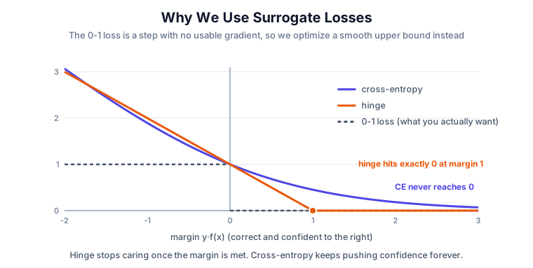
The dashed step is what you actually care about: wrong costs 1, right costs 0. It is also flat everywhere, so its gradient is zero and you cannot optimize it. Both curves above it are differentiable upper bounds you optimize instead, and the difference between them is visible at margin 1: hinge touches zero and flatlines, contributing nothing further, while cross-entropy keeps sloping down forever, still asking for more confidence on examples it already classifies correctly.
3.6 Focal Loss
For heavy imbalance, where easy negatives drown the signal (Lin et al., RetinaNet):
$$FL(p_t)=-\alpha(1-p_t)^\gamma\log(p_t)$$The \((1-p_t)^\gamma\) factor shrinks the contribution of examples the model already gets right. At \(\gamma=2\), an example at \(p_t=0.9\) contributes 100x less than it would under plain CE. Typical settings are \(\gamma=2\), \(\alpha=0.25\).
When to reach for it: dense object detection, fraud, ad click prediction, anywhere the negative-to-positive ratio runs into the thousands.
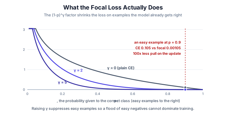
Read the right-hand side, where the easy examples live. At \(p_t=0.9\) plain cross-entropy still charges 0.105, and multiplied across a hundred thousand easy negatives that is most of your gradient. Focal loss at \(\gamma=2\) charges 0.00105 for the same example, a hundredfold reduction, while the hard examples on the left are barely touched. That selective suppression is the whole mechanism.
Trap: focal loss is not the only answer to imbalance, and leading with it can read as pattern-matching. Mention the cheaper options first: class weights,
pos_weightinBCEWithLogitsLoss, resampling, or just moving the decision threshold. Focal loss earns its place when easy negatives dominate, not merely when classes are unequal.
4. Regression
4.1 MSE (L2)
$$MSE=\frac{1}{N}\sum_i(y_i-\hat y_i)^2$$Squaring means an error of 2 costs 4 while an error of 10 costs 100, so large errors dominate. That makes MSE sensitive to outliers. Minimizing it is maximum likelihood under Gaussian noise, and it estimates the conditional mean \(E[Y \mid X]\).
4.2 MAE (L1)
$$MAE=\frac{1}{N}\sum_i|y_i-\hat y_i|$$Linear penalty, so outliers pull less. It corresponds to Laplace noise and estimates the conditional median.
Say it correctly: L1 is less sensitive to outliers than L2, not immune. Outliers still contribute. The gradient is constant in magnitude regardless of error size, which is also why L1 can oscillate near the optimum and is non-differentiable at exactly zero.
4.3 Huber
Quadratic near zero, linear in the tails:
$$L_\delta(e)=\begin{cases}\frac{1}{2}e^2 & |e|\leq\delta\\ \delta(|e|-\frac{1}{2}\delta) & |e|>\delta\end{cases}$$You get MSE’s smooth, well-scaled gradients near the optimum and MAE’s robustness far from it. The price is a hyperparameter \(\delta\) that sets where “outlier” begins.
Note: PyTorch has both
HuberLoss(delta)andSmoothL1Loss(beta). They are the same curve up to a scale factor, which matters only if you’re comparing loss values or tuning learning rate across the two.
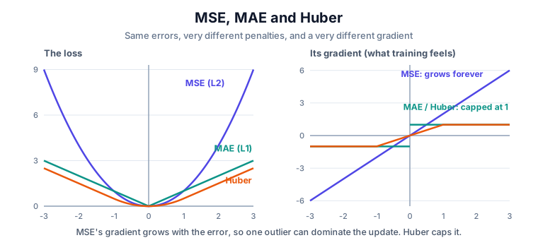
The right panel is the one that matters, because the gradient is what the optimizer actually sees. MSE’s gradient grows linearly with the error and never stops, so a single point with an error of 10 pushes ten times harder than a point with an error of 1. That is outlier sensitivity, stated mechanically. MAE and Huber cap their gradient magnitude, so no individual point can dominate the update no matter how wrong it is.
4.4 L1 / L2 as Regularization
The same norms appear as penalties on parameters rather than on predictions:
$$R_{L1}(\theta)=\lambda\sum_i|\theta_i| \qquad R_{L2}(\theta)=\lambda\sum_i\theta_i^2$$L1 drives weights to exactly zero, giving sparsity and implicit feature selection. L2 shrinks weights smoothly toward zero without eliminating them, spreading influence across correlated features. L2 is usually called weight decay, though the equivalence is exact only for plain SGD, which is why AdamW decouples them.
Trap: don’t say “L1 and L2 are loss functions.” Say: “L1 and L2 are norms. Used on residuals they’re prediction losses; used on parameters they’re regularizers.” That one sentence signals you understand the difference.
5. Ranking
Ranking cares about relative order, not absolute labels. A model scores items with \(s(x)\) and the goal is that relevant items outrank irrelevant ones. This covers search, recommendation, and ads.
Why ranking data is cheap. You never need an absolute relevance score, only a relative signal, and binary is enough. For face verification you only need to know which image pairs are the same person. Clicks, purchases, and dwell time give you that signal for free. This is exactly why ranking objectives dominate search and recommendation, where absolute relevance labels are expensive, inconsistent between annotators, and stale within a month.
The taxonomy (know this shape, it’s the question):
| Approach | Unit | Optimizes |
|---|---|---|
| Pointwise | one item | predicted relevance, as regression or classification |
| Pairwise | a pair | \(s_i>s_j\) when \(i\) is preferred |
| Listwise | the whole list | a list metric such as NDCG |
Pairwise reframes “is this item good?” as “should A outrank B?” Two standard forms:
$$L_{margin}=\max(0,m-y(s_i-s_j)) \qquad L_{logistic}=-\log\sigma(s_i-s_j)$$The margin version stops once \(s_i \geq s_j+m\). The logistic version keeps pushing the gap wider with diminishing returns, and is the Bradley-Terry preference model. Note this is the same mathematical shape that DPO uses on preferred vs rejected responses.
Listwise (ListNet, ListMLE, LambdaRank/LambdaMART) optimizes the full list. LambdaRank’s trick is weighting each pair by how much swapping it would change NDCG, which smuggles a non-differentiable ranking metric into the gradient.
Trap: “why not just train pointwise regression on relevance labels?” Because ranking metrics only depend on order, and pointwise loss wastes capacity fitting absolute scores nobody looks at. Getting all scores wrong by a constant is free in NDCG and expensive in MSE.
6. Contrastive and Metric Learning
Here the output is an embedding space, not a prediction. Similar things should land close together, dissimilar things far apart. This powers semantic search, retrieval, face recognition, RAG, and CLIP-style multimodal models.
The defining property: you only care about relative distances in that space, never the coordinate values themselves. That is also why contrastive learning needs no labels. If you can construct a pair you know is related, you have a training signal, which is what makes it the workhorse of self-supervised learning.
6.1 Contrastive (pair)
With \(y=1\) for similar, \(y=0\) for dissimilar, and distance \(d\):
$$L=y\,d^2+(1-y)\max(0,m-d)^2$$Similar pairs are pulled together; dissimilar pairs are pushed apart only until they exceed margin \(m\). Without that margin, the model would waste capacity pushing already-distant negatives further apart forever.
6.2 Triplet
Anchor \(a\), positive \(p\), negative \(n\):
$$L=\max(0,\,d(a,p)-d(a,n)+m)$$The positive must be closer than the negative by at least \(m\).
Trap: the loss is the easy half; mining is the hard half. Random triplets are satisfied almost immediately and produce zero gradient, so training stalls. You need semi-hard or hard negative mining. If you mention triplet loss without mentioning mining, expect that as the follow-up.
6.3 InfoNCE / Multiple Negatives
Use every other item in the batch as a negative:
$$L=-\log\frac{\exp(sim(q,p^+)/\tau)}{\sum_j\exp(sim(q,p_j)/\tau)}$$A batch of \(N\) gives you \(N-1\) negatives for free, with no mining pipeline. This is why large batches matter so much for contrastive training, and it’s the objective behind CLIP and most dense retrievers.
Look closely: this is softmax cross-entropy where the “classes” are the candidates in the batch. The temperature \(\tau\) controls sharpness. Small \(\tau\) concentrates the gradient on the hardest negatives; too small and training destabilizes.
6.4 Cosine Similarity
$$\cos(z_1,z_2)=\frac{z_1\cdot z_2}{\|z_1\|\|z_2\|}$$Use it when direction carries the meaning and magnitude doesn’t, which is the normal situation for text embeddings. HingeEmbeddingLoss expresses the same similar/dissimilar idea using Euclidean distance instead of cosine similarity.
6.5 Where Positives Come From
The loss is the easy half. The design question interviewers actually probe is how you decide two samples are similar when nobody labeled them. Three standard answers:
| Source of positives | How it works | Trade-off |
|---|---|---|
| Augmentation | Two views of the same sample: crop, mask, token dropout | The self-supervised default (SimCLR). The space becomes invariant to whatever you augment, so the augmentation choice is the inductive bias |
| Input-space neighbors | Treat the \(N\) nearest samples as similar | Gives a smooth latent space, but you need a meaningful metric in input space to begin with |
| Labels | Same class implies similar | Cheap when labels exist, but crude: two samples of one class can be genuinely dissimilar, which leaves the space less smooth |
Worth naming in an interview: FaceNet used triplet loss for face embeddings, SimCLR builds positives from augmentations, and CLIP uses InfoNCE over cosine similarities between image and text, where the only supervision is which caption shipped with which image.
6.6 Contrastive vs Ranking
They overlap and interviewers like the distinction. Ranking asks put preferred items above others; contrastive learning asks build a space where related things are close. A contrastive objective is frequently used to train a retrieval model that is then evaluated with ranking metrics. Not mutually exclusive.
7. KL Divergence
How far distribution \(Q\) is from \(P\):
$$D_{KL}(P\|Q)=\sum_x P(x)\log\frac{P(x)}{Q(x)}$$It is \(\geq 0\), zero only when \(P=Q\), and not symmetric, so it is a divergence and not a distance.
Forward vs reverse is the question that separates people who’ve read about KL from people who’ve used it:
| Behavior | Result | |
|---|---|---|
| Forward \(D_{KL}(P\|Q)\) | mass-covering | \(Q\) spreads to cover all of \(P\), including low-density regions |
| Reverse \(D_{KL}(Q\|P)\) | mode-seeking | \(Q\) collapses onto one mode of \(P\) |
Forward KL is infinite wherever \(P>0\) and \(Q=0\), so \(Q\) must cover everything. Reverse KL is happy to ignore whole modes, which is why VAEs using reverse KL produce blurry, mode-collapsed samples.
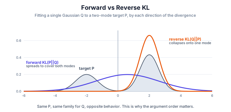
Both fits are the best single Gaussian available, computed by minimizing each direction numerically against the same target. Forward KL lands at \(\mu=0.6,\ \sigma=2.0\): it smears across both modes and puts real probability mass in the valley between them, where the target has almost none. Reverse KL lands at \(\mu=2.0,\ \sigma=0.6\), which is exactly the right mode’s own parameters; it fits that mode perfectly and pretends the other does not exist. Same target, same family, opposite failure. Which one you want depends on whether missing a mode or hallucinating between modes is the worse outcome for your application.
Shows up in: knowledge distillation, VAEs, RLHF policy constraints, and any distribution matching.
Trap:
nn.KLDivLossexpects the input as log-probabilities and the target as probabilities (unless you setlog_target=True). Passing raw probabilities gives a wrong number with no error. Also note cross-entropy equals entropy plus KL, so with a fixed target distribution, minimizing CE and minimizing KL are the same optimization.
8. LLM Losses
8.1 Pretraining: Token Cross-Entropy
Autoregressive models predict each token from its prefix:
$$L=-\frac{1}{T}\sum_{t=1}^{T}\log P(x_t \mid x_{\lt t})$$Given “The cat sat on the ___”, if the true token is “mat”, the loss is \(-\log P(\text{mat})\). At \(P=0.9\) it’s small; at \(P=0.01\) it’s large. That’s all pretraining is: cross-entropy over the vocabulary, applied at every position.
Teacher forcing means the model conditions on the ground-truth prefix during training, not its own generations. This makes training parallel across positions, but creates exposure bias: at inference the model conditions on its own output, including its own mistakes, a distribution it never trained on.
8.2 SFT
Same token cross-entropy, but the loss is masked to the response tokens. Prompt tokens are set to -100 so CrossEntropyLoss skips them via ignore_index.
Trap: forgetting the mask trains the model to generate prompts as well as answers. It’s a real bug with a plausible-looking loss curve, which is exactly what makes it a good interview question.
8.3 Distillation
The student matches the teacher’s full distribution rather than just the hard label:
$$L = \alpha\, T^2 D_{KL}(P_{teacher}^{T}\|P_{student}^{T}) + (1-\alpha)\,CE(y, P_{student})$$A teacher saying cat 0.70, dog 0.25, car 0.05 communicates that cats resemble dogs and not cars. That “dark knowledge” is the entire point, and a one-hot label throws it away.
Temperature \(T>1\) softens both distributions to expose the small probabilities. The \(T^2\) factor is there because softening scales the gradients down by \(1/T^2\), and without it your learning rate would need retuning per temperature.
8.4 DPO
Given a prompt \(x\), preferred \(y_w\), rejected \(y_l\), and a frozen reference model:
$$L=-\log\sigma\left(\beta\left[\log\frac{\pi_\theta(y_w \mid x)}{\pi_{ref}(y_w \mid x)}-\log\frac{\pi_\theta(y_l \mid x)}{\pi_{ref}(y_l \mid x)}\right]\right)$$This is the pairwise logistic loss from section 5, with the score being the log-ratio against the reference. DPO’s contribution is showing that the RLHF objective has a closed-form optimum you can hit with a supervised loss, so no reward model and no RL loop are needed. \(\beta\) controls how far the policy may drift.
8.5 RLHF
A reward model scores generations, and a KL penalty keeps the policy near the reference:
$$R_{total}=R_{reward}-\beta D_{KL}(\pi_\theta\|\pi_{ref})$$Maximize reward, but don’t wander. Without the KL term the policy reward-hacks: it finds degenerate text that scores well under an imperfect reward model and is useless to humans.
9. Perplexity
Not a training loss. It’s an evaluation metric that is a monotone transform of cross-entropy:
$$PPL=e^{L}$$where \(L\) is average token cross-entropy in nats. So \(L=2 \Rightarrow PPL\approx7.39\), loosely readable as “the model is as uncertain as if choosing uniformly among 7.39 tokens.”
Trap: perplexity is only comparable across models with the same tokenizer and the same evaluation data. Different tokenizers change the number of tokens a text occupies, which changes per-token loss, which changes perplexity. Cross-model perplexity comparisons in papers are frequently apples-to-oranges.
10. How to Answer “Which Loss Would You Use?”
Never answer with just a name. Walk the ladder, out loud, in about thirty seconds:
- What’s the task? Classification, regression, ranking, retrieval, generation.
- What’s the target? Continuous value, class, probability, relative preference, embedding, token sequence.
- What’s wrong with the data? Outliers, class imbalance, label noise, multiple labels per example, a need for calibrated probabilities.
- What does the loss actually optimize? Tie it back to the metric you’ll be judged on.
- When does it fail? This is the step that separates senior from junior answers.
A good answer sounds like:
“Binary classification, so BCE on logits, since it directly optimizes the likelihood of the correct class. The classes are 1000:1 imbalanced, so I’d start with
pos_weightrather than focal loss, because it’s one argument and easier to reason about. If easy negatives still dominate the gradient I’d move to focal with \(\gamma=2\). And I’d watch calibration, because reweighting distorts the output probabilities, which matters if a downstream threshold depends on them.”
Task, loss, reason, failure mode. Anyone can name a loss; the reason and the failure mode are what’s being tested.
11. Rapid-Fire Q&A
Why cross-entropy instead of MSE for classification? With a sigmoid or softmax output, MSE gives a non-convex surface and gradients that vanish exactly when the model is confidently wrong, which is when you most need a signal. CE’s gradient is proportional to \((p-y)\), so it stays strong.
Why is the log there? It turns products of likelihoods into sums (numerically tractable) and makes confident mistakes arbitrarily expensive. Minimizing negative log-likelihood is maximum likelihood estimation.
MSE vs MAE in one line? MSE estimates the conditional mean and punishes outliers; MAE estimates the conditional median and tolerates them.
Can loss be negative? Not for CE, MSE, or hinge, which are bounded below by zero. Yes for continuous-target losses involving log-densities, where a density can exceed 1. A negative CE means a bug.
Loss is going down but the metric isn’t. Why? Your loss is a proxy for the metric, not the metric. Common cases: accuracy on imbalanced data while the model predicts the majority class; NDCG while you optimize pointwise MSE; BLEU while you optimize token CE.
Why can’t we optimize accuracy directly? It’s piecewise constant, so its gradient is zero almost everywhere. Same reason we don’t put argmax in a loss.
What does reduction change? 'mean' averages over the batch, 'sum' doesn’t. With 'sum', your effective learning rate scales with batch size, which is a classic silent bug when someone changes the batch size.
Weighted loss vs resampling for imbalance? Weighting keeps every example and changes its gradient contribution; resampling changes the data the model sees. Weighting is cheaper and deterministic; resampling can work better when the imbalance is extreme enough that weights become unstable.
Why does contrastive training need big batches? In InfoNCE the negatives come from the batch, so batch size is the number of negatives, which directly sets the difficulty of the task.
Two models, same architecture, different loss. Which is better? Unanswerable from the loss values alone unless the loss is identical and the data identical. Compare on the evaluation metric.
The Idea Underneath
Every loss above is answering one question: what does “good” mean here?
The optimizer has no idea whether an output is a correct label, a useful embedding, a well-ordered result list, or a helpful answer. It only descends a gradient. The loss function is where you define what you actually want, and every failure mode in this post is what happens when that definition doesn’t quite match the thing you cared about.
Pick the loss that encodes your real objective. Then check what it quietly ignores.