Companion to what you must know about NLP and LLMs. That post treats embeddings as one step in NLP’s history. This one treats them as what they actually are now: the layer underneath search, ads ranking, recommendation and RAG, most of which has nothing to do with language.
If you had to point at one idea that shows up in nearly every production ML system, it’s this one. Ads ranking, recommendation, semantic search, RAG, dedup, fraud rings, face recognition. All of them come down to turning things into vectors and then asking which vectors are close.
Say it like this: an embedding is a learned lookup table that turns an ID into a vector, arranged so that similar things land near each other.
That’s the whole concept. The rest is how you learn the table and how you search it.
1. What It Actually Is
Start with something concrete. You have 10 million products and you want the model to understand them.
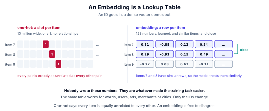
One-hot gives each product a 10-million-long vector that’s all zeros except one 1. It’s honest and useless: no two products are related, and your first weight matrix would have 10 million rows.
An embedding gives each product a row in a table, maybe 128 numbers wide. Product 5,331,208 is just row 5,331,208. Look it up, get a vector, feed it forward.
The numbers in that table are learned, not designed. Nobody decides that dimension 47 means “outdoorsy”. You define a task, train, and the table arranges itself so the task gets easier. Whatever structure ends up in there is whatever helped.
Three things follow, and they’re why embeddings took over:
- Dense and small. 128 numbers rather than 10 million slots.
- Similarity is free. Two products used in similar ways end up nearby, so distance becomes meaningful without anybody labelling pairs.
- Generalization. A product with few interactions still lands near similar products, so the model can say something sensible about it.
Trap: “embeddings are for text.” The mechanism has nothing to do with language. A user ID, a product, an ad, a city, a merchant category all get embedded the same way, and in most production recsys those tables hold more parameters than the rest of the model combined.
2. The Map
| How you build it | What it learns from | Where you see it |
|---|---|---|
| Matrix factorization | an interaction matrix | classic recsys, still a solid baseline |
| word2vec style | co-occurrence in a sequence | words, and also items in a session |
| Supervised by-product | any classifier’s hidden layer | categorical features inside a bigger model |
| Two-tower / dual encoder | pairs that belong together | ads and recsys retrieval, at scale |
| Encoder models | sentence pairs, contrastively | semantic search, RAG |
| LLM-derived | a big pretrained decoder | strong general-purpose text vectors |
Say it like this: every method here is the same trick with a different training signal. Put things that belong together close, and let everything else fall where it falls.
3. How People Actually Build Them
3.1 Matrix factorization, where this started
Before anyone said “embedding”, recommender systems had a giant sparse matrix: users down the side, items across the top, ratings in the cells, and almost everything missing.
Factorize it into two thin matrices, one row per user and one row per item, so their product roughly reconstructs the ratings you do have:
$$R \approx U V^{T}$$Say it like this: matrix factorization invents a small set of hidden traits, then describes every user and every item by how much of each trait they have.
Those rows are embeddings. The model never sees a genre, but latent dimensions arrive that behave like genres, because that’s the compression that explains the data.
Pros: simple, fast, interpretable-ish, still a real baseline. Cons: it only knows IDs it saw during training, so a brand new item has no row at all. That’s the cold start problem, and it’s the reason content features exist.
3.2 word2vec style, on things that aren’t words
The NLP post covers this for text. The part worth repeating here is that the trick isn’t about language at all.
Swap “words in a sentence” for “items in a browsing session” and the same algorithm gives you item embeddings. Products bought together end up close, because they appear in the same contexts. This shipped widely as item2vec and its relatives, and it’s a genuinely good answer when you have sequences of behaviour and no labels.
3.3 Embeddings inside a supervised model
You don’t need a dedicated embedding job. Put an embedding layer in any model and the table trains along with everything else.
This is how categorical features work in deep recsys and ads models. user_id, ad_id, publisher, device, country all get tables, the model trains on click prediction, and the tables fill up with whatever helps predict clicks.
Two practical problems come with this:
High cardinality. 500 million user IDs times 128 dimensions is 64 billion parameters for one feature. The usual answer is the hashing trick: hash the ID into a fixed number of buckets and accept that some IDs collide. Collisions cost a little accuracy and save an enormous amount of memory.
Cold start. New ID, untrained row. You fall back to content features (what kind of thing is it) rather than identity, which is why production models carry both.
Trap: “how big is the model?” For a deep recsys or ads model the honest answer is usually “the embedding tables”, and it’s not close. The dense layers might be tens of millions of parameters while the tables are tens of billions. That shapes everything about how it’s served and sharded.
3.4 Two-tower, the production workhorse
This is the one to know cold, because it’s how large-scale retrieval actually works.
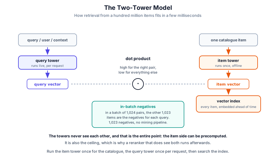
You have two encoders. One turns the query (or user, or context) into a vector. The other turns a candidate item into a vector. Train them so that matching pairs have a high dot product and everything else doesn’t.
Say it like this: two towers, one for the question and one for the answer, trained so the right pairs point the same way.
The whole point is that the towers never touch. Because the item tower only looks at the item, you can run it once, offline, for your entire catalogue, and store the results in a vector index. At request time you run only the query tower, one forward pass, then search the index. That’s what makes it feasible to retrieve from a hundred million items in a few milliseconds.
Where the negatives come from. You have positives (this user clicked this ad) and almost no explicit negatives. The standard trick is in-batch negatives: in a batch of 1,024 pairs, the other 1,023 items serve as negatives for each query. One batch gives you a thousand negatives for free, and the loss is just softmax cross-entropy over the batch (InfoNCE, from the loss post).
Trap: in-batch negatives are sampled by popularity, because popular items appear in more batches. Left alone, the model learns to suppress popular items in a way that doesn’t reflect reality. Production systems apply a logQ correction, subtracting the log sampling probability from the logits. Knowing that this correction exists is a strong signal you’ve actually trained one of these.
Cons worth saying out loud: the two towers can’t see each other, so no feature can depend on the query and item jointly. That ceiling is real, and it’s exactly why retrieval is followed by a reranker that can look at both together.
3.5 Encoder models and LLM-derived embeddings
For text, a bidirectional encoder fine-tuned on sentence pairs gives you general-purpose embeddings. Sentence-transformers made this the default, and it’s still what most RAG stacks run.
More recently, embeddings extracted from large decoder models have taken the top of the benchmarks. They’re better, and they’re bigger and slower, which is a normal tradeoff rather than a free win. For a lot of production retrieval a 384-dimensional small model is the right answer, because you’re going to store a hundred million of them and search them in 10ms.
4. Turning a Model Into One Vector
A transformer gives you one vector per token. You need one vector for the whole text. Something has to collapse them.
| Method | How | Reality |
|---|---|---|
| CLS token | use the special first token’s vector | needs to be trained for it, poor off the shelf |
| Mean pooling | average all token vectors | the reliable default |
| Last token | the final position’s vector | used for decoder-derived embeddings, since only it has seen everything |
Say it like this: mean pooling is the boring choice that usually wins.
Trap: taking
CLSoff a plain pretrained BERT and using it as a sentence embedding. It was never trained to summarize the sentence, so it’s often worse than averaging. This is a genuinely common bug and it’s why Sentence-BERT exists.
5. Comparing Two Vectors
Three measures, and the difference matters more than people expect.
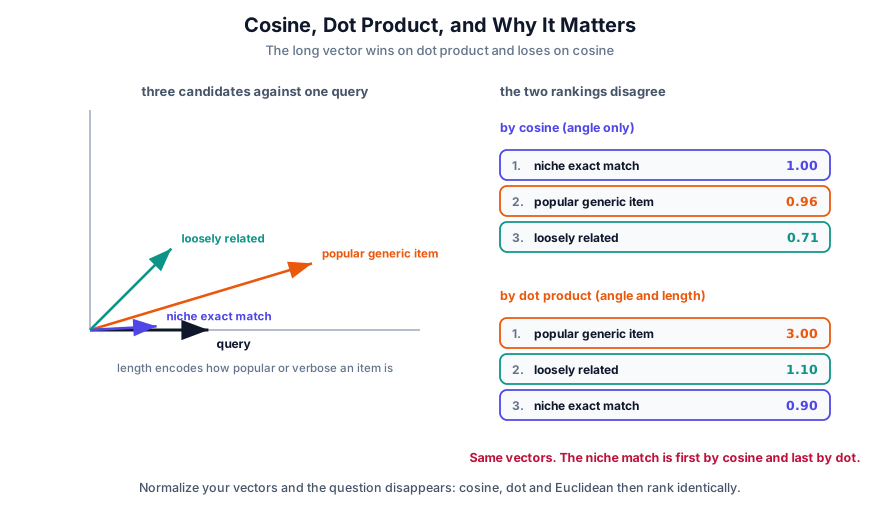
Those are real numbers from three vectors. The niche exact match ranks first by cosine and last by dot product, purely because it’s a short vector. Nothing about the angle changed; only whether length was allowed to count.
$$\cos(a,b)=\frac{a\cdot b}{\lVert a\rVert\,\lVert b\rVert} \qquad a\cdot b=\sum_i a_ib_i \qquad \lVert a-b\rVert$$- Cosine is the angle only. Length is ignored entirely.
- Dot product is the angle and the lengths. A long vector scores higher against everything.
- Euclidean is straight-line distance, which mixes both in a different way.
Say it like this: cosine asks which direction, dot product asks which direction and how loudly.
The fact that resolves most confusion: if your vectors are L2-normalized, all three rank identically. Cosine and dot become the same number, and Euclidean distance becomes a monotone function of it. So “cosine vs dot” is only a real question when your vectors are not normalized.
Which means the actual question is: do you want magnitude to count?
- In recommendation, vector length often encodes popularity, and a dot product will quietly favour popular items. Sometimes that’s exactly right, sometimes it’s a bias you need to remove.
- For text similarity you almost always normalize, because a longer document shouldn’t automatically be more similar to everything.
Trap: switching from dot to cosine on an index built for dot. Maximum inner product search and nearest-neighbour search are different problems, because inner product isn’t a proper distance metric (a vector isn’t closest to itself under dot product). Some index types handle only one. Normalize first and the distinction disappears.
6. Searching a Billion Vectors
You have 100 million embeddings and a query. Comparing against all of them is exact and far too slow.
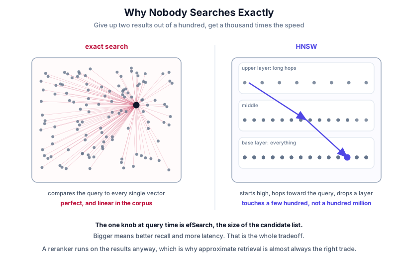
Approximate nearest neighbour trades a sliver of correctness for orders of magnitude of speed. You accept finding 98 of the true top 100 in exchange for a 1000x speedup, and in a system that reranks afterwards that trade is almost always worth it.
| Index | Idea | Trade |
|---|---|---|
| Flat | compare everything | exact, and linear in the corpus |
| IVF | cluster vectors, search only the nearest few clusters | tune nprobe for recall against speed |
| HNSW | a layered graph you walk greedily toward the query | fast and high recall, but memory hungry |
| PQ | chop each vector into pieces and store a codebook ID per piece | huge compression, approximate distances |
HNSW is the default for a reason. Build a graph where each vector links to its neighbours, with sparse long-range links in upper layers. To search, start at the top, greedily hop toward the query, drop a layer, repeat. You touch a few hundred vectors instead of a hundred million.
Say it like this: HNSW is a road network with motorways on top and side streets underneath, and searching is just always driving toward the destination.
The one knob that matters at query time is efSearch, the size of the candidate list. Bigger means higher recall and more latency. That’s your recall-latency dial and it’s what you tune in production.
Product quantization is the memory answer. 100 million vectors at 768 float32 dimensions is 307 GB, which does not fit anywhere convenient. PQ splits each vector into sub-vectors, replaces each with the nearest entry in a small learned codebook, and stores one byte per piece. The same data lands under 10 GB, at a real but usually acceptable accuracy cost.
6.1 What you actually run
Almost nobody implements HNSW themselves. Here’s the landscape, and the distinction that matters is library or database.
| What it is | When it’s right | |
|---|---|---|
| FAISS (Meta) | the library everyone benchmarks against. Flat, IVF, HNSW, PQ and combinations of them | you want an index inside your own service and you’ll handle storage yourself |
| ScaNN (Google) | similar scope, strong quantization | same niche as FAISS, often faster at high recall |
| hnswlib | a small, fast HNSW-only implementation | you want exactly HNSW and nothing else |
| pgvector | vector columns in Postgres | you already run Postgres. Usually the right answer well past the scale people assume |
| Pinecone, Milvus, Qdrant, Weaviate | purpose-built vector databases | you need filtering, live updates, replication and an API without building them |
| Elasticsearch, OpenSearch, Vespa | search engines that added vectors | you want hybrid search, keyword and vector scored together, in one system |
Say it like this: FAISS gives you an index. A vector database gives you an index plus everything around it.
FAISS is a library: it builds an index in memory and searches it, and that’s the job. No persistence story, no metadata filtering, no incremental updates, no replication. If you want those you write them, which is fine when the index fits on one machine and rebuilds nightly. It also exposes index types as compact strings like IVF4096,PQ64, which is worth recognizing, since that one line tells you the whole storage and accuracy tradeoff someone picked.
A vector database is an ANN index plus the production concerns: persistence, filtered search (find similar and price under 50), updates without a full rebuild, sharding, replication. The interesting engineering there is mostly in filtering and incremental updates, not in the distance computation, which is a solved problem.
Trap: reaching for a new database when a column would do. If you have ten million vectors and already run Postgres,
pgvectorwith an HNSW index is very likely enough, and it means your vectors sit next to the data you’re going to filter on anyway. “We need a vector DB” is a conclusion, not a starting point.
One more thing worth knowing: hybrid search. Dense retrieval is bad at exact matches, because “error code E4021” has no useful semantics and an embedding will happily return something conceptually similar. Keyword search nails it. Running BM25 and vector search together and fusing the rankings beats either alone, which is a nice result given that BM25 is a direct descendant of TF-IDF. The oldest idea in the stack is still earning its place.
7. The Practical Bits
Dimensionality. 384 is fine for a lot of retrieval, 768 is the common default, 1536 and above is usually more than you need. Cost is linear in dimensions for both storage and search, so this is a real budget decision rather than a “bigger is better” one.
Matryoshka embeddings are worth knowing. Trained so that the first 256 dimensions are independently useful, they let you truncate a 1536-dimensional vector down and keep most of the quality. Retrieve cheaply with 256, rerank precisely with the full vector.
Re-embedding is the hidden cost. Change your embedding model and every vector you’ve ever stored is now meaningless, because the new model’s space is unrelated to the old one. For a hundred million documents that’s a genuine migration with a dual-index period. You cannot mix embeddings from two models in one index.
Hard negatives decide quality. Random negatives are too easy: a query about kidney function against a random news article teaches the model nothing. Mine negatives that are almost right, usually by retrieving with the current model and taking high-ranked wrong answers. This is normally the difference between a mediocre retriever and a good one.
Measure with recall@k, and measure two different things: how good the embeddings are (against exhaustive search) and how good the index is (against exact search on the same embeddings). Conflating those two is how people end up tuning the index when the model was the problem.
8. Rapid-Fire Q&A
What is an embedding, in one sentence? A learned lookup table from an ID or an input to a dense vector, arranged so similar things end up close.
Cosine or dot product? If the vectors are L2-normalized they rank identically, so it doesn’t matter. If they aren’t, dot product lets magnitude count, which usually means popularity. Text similarity normalizes; recommendation sometimes deliberately doesn’t.
Why a two-tower model instead of one model over the pair? Because the towers are independent, you can embed the whole catalogue offline and only run the query tower live. A joint model would need a forward pass per candidate, which is impossible at retrieval scale. You use the joint model afterwards, as the reranker.
Where do the negatives come from in two-tower training? In-batch negatives: everything else in the batch. Then a logQ correction, because in-batch sampling is biased toward popular items.
Why is a recsys model mostly embedding tables? Because every high-cardinality categorical feature gets a row per value. Millions of users times a hundred dimensions dwarfs the dense layers.
What do you do about a brand new item? Content features instead of identity, so the model can place it by what it is rather than by who interacted with it. Pure ID embeddings cannot cold start.
Mean pooling or CLS? Mean pooling unless the model was explicitly trained to use CLS. Plain BERT’s CLS is not a sentence embedding.
How does HNSW work? A layered graph with long-range links on top and local links below. Start high, greedily move toward the query, drop down, repeat. efSearch trades recall against latency.
Why product quantization? Memory. Storing a hundred million high-dimensional float vectors is hundreds of gigabytes; PQ compresses that by an order of magnitude with approximate distances.
Can you mix embeddings from two different models? No. Different models produce unrelated spaces, so distances between them are meaningless. Changing models means re-embedding everything.
What actually makes a retriever good? Hard negatives, more than architecture. Random negatives train a model that can only tell apart things that were never confusable.
FAISS or a vector database? FAISS is a library that builds and searches an index, with no persistence, filtering or replication. A vector database wraps an index in those things. If you already run Postgres, pgvector covers a surprising amount of ground before you need either.
When does dense retrieval fail? Exact strings. Error codes, SKUs, names and IDs have no useful semantics, so an embedding returns something conceptually near instead of the thing you asked for. Hybrid search with BM25 fixes it.
The Idea Underneath
Every method in this post does the same thing: it turns identity into geometry.
A product ID means nothing. It’s a number, and number 5,331,208 is not “near” number 5,331,209 in any useful sense. An embedding replaces that meaningless label with a position, and once things have positions, near becomes a question you can answer with arithmetic.
That’s the whole reason this layer sits under so much of modern ML. Search, recommendation, retrieval, dedup and clustering are all the same question once you’ve done it: what else is near this? The hard part was never the searching. It was learning a space where nearness means something.